A plausible model gives the wrong answer
Page status: introductory counterexample with executable scalar and multiconductor evidence; independent mathematical review remains open.
By the end of this lesson, you will be able to check a parallel-branch replacement, recover its member currents, and derive a correct aggregate rating for a fixed scalar example. You need Ohm's law and inequalities; the calculation runs with standard-library Python.
Predict before calculating
Two lines connect the same buses. Each is rated for 100 A, but one has ten times the conductance of the other. Can the pair safely carry 200 A?
Write down a prediction, including how you expect the current to divide. First examine the current split in this resistive model:
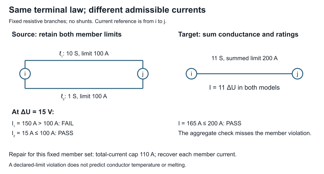
Assume fixed, uncoupled, series-only resistive branches with common endpoints, no shunts, and no other constraints in this local calculation. Consider two scalar resistive branches $\ell_1 i j$ and $\ell_2 i j$ with intrinsic impedances
\[Z_{\ell_1}=0.1\ \Omega,\qquad Z_{\ell_2}=1.0\ \Omega,\]
and member current limits
\[I^{\max}_{\ell_1}=I^{\max}_{\ell_2}=100\ \mathrm{A}.\]
Writing $\Delta U=U_i-U_j$ and $Y_{\ell}=Z_{\ell}^{-1}$, the terminal currents are
\[I_{\ell_k i j}=Y_{\ell_k}\Delta U,\qquad k\in\{1,2\}.\]
Here $k$ identifies a member, and positive current follows the stored orientation from $i$ to $j$.
Replacing the pair by one branch with
\[Y_{\mathrm{eq}}=Y_{\ell_1}+Y_{\ell_2}=11\ \mathrm{S}\]
is exact for the unconstrained total terminal-current relation. It does not follow that the replacement is exact for a decision problem with member limits.
The feasible sets differ
The source model requires both inequalities
\[|Y_{\ell_1}\Delta U|\le I^{\max}_{\ell_1},\qquad |Y_{\ell_2}\Delta U|\le I^{\max}_{\ell_2}.\]
Hence its admissible voltage-drop magnitude is
\[|\Delta U|\le \min\left\{\frac{I^{\max}_{\ell_1}}{|Y_{\ell_1}|}, \frac{I^{\max}_{\ell_2}}{|Y_{\ell_2}|}\right\} =10\ \mathrm{V}.\]
A tempting aggregate construction assigns the equivalent branch the summed rating, $I^{\max}_{\mathrm{eq}}=200\ \mathrm{A}$. It admits
\[|\Delta U|\le \frac{200}{11}\ \mathrm{V}\approx18.18\ \mathrm{V}.\]
At the witness $\Delta U=15\ \mathrm{V}$, the equivalent branch carries $165\ \mathrm{A}$ and satisfies its aggregate limit. Recovery gives
\[I_{\ell_1 i j}=150\ \mathrm{A},\qquad I_{\ell_2 i j}=15\ \mathrm{A},\]
so the source violates the $\ell_1$ limit. The target feasible set is therefore an outer relaxation of the source feasible set.
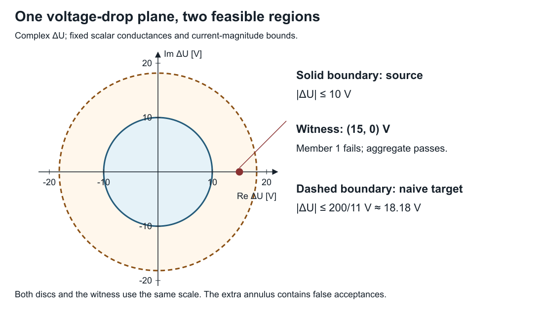
The figure is generated by experiments/render_parallel_feasible_set_card.py. The retained and aggregate regions are discs in the complex $\Delta U$ plane, plotted in volts on identical horizontal and vertical scales. The point $(15,0)$ lies in the target’s extra region. No weighted or coupled constraint is represented in this scalar plot.
Repair the aggregate
The source requires $|\Delta U|\le10\ \mathrm V$. Since the total current is $11\Delta U$, the exact aggregate current-magnitude cap for this fixed scalar model is
\[I^{\max}_{\mathrm{eq,exact}}=11\times10=110\ \mathrm A.\]
This rating reproduces the local member-constrained voltage-drop set. Both members remain recoverable from $\Delta U$ and their retained admittances. At the cap, member currents are 100 A and 10 A. The weakly conducting member cannot use its remaining capacity independently of the common voltage drop.
A correct reduction can therefore be useful. Its rating must be derived from what the study constrains. The 110 A cap belongs to this fixed member set; opening a member changes both the equivalent admittance and the cap. Retain member identities and a state-dependent construction if outages are decisions.
A decision problem exposes the gap
The same mechanism changes an optimum in a two-bus maximum-served-load model. Let the parallel members have
\[(b_{\ell_1},b_{\ell_2})=(1000,100)\ \mathrm{MW/rad},\qquad (F^{\max}_{\ell_1},F^{\max}_{\ell_2})=(100,100)\ \mathrm{MW},\]
with $F_{\ell i j}=b_\ell\delta_{ij}$, nonnegative $\delta_{ij}$, and served power equal to total flow. The source model keeps both member laws and both limits. The naïve target uses $b_{\mathrm{eq}}=1100$ MW/rad and $F^{\max}_{\mathrm{eq}}=200$ MW.
| Formulation | Maximum served power | $\delta_{ij}$ | Active restriction |
|---|---|---|---|
| source members | 110 MW | 0.1 rad | $F_{\ell_1 i j}\le100$ MW |
| naïve aggregate | 200 MW | $2/11$ rad | summed 200 MW rating |
| aggregate relation with exact lifted member constraints | 110 MW | 0.1 rad | recovered $F_{\ell_1 i j}\le100$ MW |
The displayed exact lifted formulation retains every member law and both member limits:
\[F_{\ell i j}=b_\ell\delta_{ij},\qquad F_{\ell i j}\le F^{\max}_\ell \quad\text{for every }\ell,\]
alongside the aggregate terminal relation. It therefore reproduces the source feasible set and optimum without pretending that a summed scalar rating is exact. This computed comparison is claim TR-PAR-003. JuMP and Ipopt produce the machine-readable result in experiments/generated/parallel-opf-comparison.json; the analytic values above also provide a solver-independent check.
Here $b_{\ell_2}=0.1b_{\ell_1}$ and the ratings are equal, so the $\ell_2$ limit is actually implied by the $\ell_1$ limit and can be certifiably pruned. Keeping both in the table isolates the lifting argument from presolve; the next case implements the pruned formulation explicitly.
The Multiconductor parallel AC decision case extends this comparison to coupled complex conductor equations, phase-to-neutral constant power, and voltage-magnitude constraints.
Run the calculation
From the repository root, with Python 3 installed:
python3 experiments/lessons/parallel_members.pyThe script uses exact rational arithmetic for this scalar calculation:
first member current: 150 A
second member current: 15 A
aggregate current: 165 A
summed-rating check: pass
recovered member checks: fail
exact voltage-drop magnitude cap: 10 V
exact aggregate current-magnitude cap for this state: 110 A
No power-flow solver is involved. The calculation checks the branch laws and ratings specified above. It does not model temperature, protection operation, voltage-dependent impedance, or uncertainty in the ratings. The later AC case adds network equations and load constraints.
Run the boundary and outage checks with:
python3 experiments/lessons/parallel_members.py --check
python3 experiments/lessons/parallel_members.py --drop 10
python3 experiments/lessons/parallel_members.py --open-member first
Change one assumption
- Increase the first member's rating to 200 A. Predict the exact aggregate cap, then run
--limit-first 200. Which member binds? - Open the first member while retaining a 15 V drop. Predict the remaining current and explain why the old equivalent is invalid.
- Reverse the voltage drop with
--drop -15. Which feasibility conclusions change, and which depend only on magnitude? - Write the exact aggregate rating for arbitrary positive real admittances $Y_1,Y_2$ and positive member ratings. State why the same formula is not automatically a conventional multiconductor rating.
Check your reasoning
With the first rating at 200 A, the voltage-drop cap becomes 20 V and the aggregate cap 220 A; the first member still binds. With that member open, the remaining conductance is 1 S, the current at 15 V is 15 A, and the remaining rating is 100 A. Reversing the drop reverses both currents without changing the magnitude-limit checks.
For the fixed positive-real scalar model,
\[I^{\max}_{\mathrm{eq,exact}} =(Y_1+Y_2)\min\left\{\frac{I^{\max}_1}{Y_1}, \frac{I^{\max}_2}{Y_2}\right\}.\]
For multiple conductors, member constraints act on vector-valued currents. Their inverse images need not have the form of one conventional aggregate rating. The extension below states that set explicitly.
Preservation contract
| Contract field | Value |
|---|---|
| source | two identified parallel branches with individual limits |
| target | one equivalent branch with summed admittance and rating |
| preconditions | common endpoints and voltage coordinates; linear branch laws |
| preserves | unconstrained total terminal current as a function of $\Delta U$ |
| does not preserve | the member-constrained feasible set |
| forgets | member identity and independent outage, maintenance, or investment state |
| recovery | $I_{\ell_k i j}=Y_{\ell_k}\Delta U$ if member admittances remain available |
| classification | outer/relaxed for this rating construction |
This counterexample does not say that parallel aggregation is never useful. It says that an aggregate rating needs its own derivation relative to the intended observation or decision set. Choosing a tighter equivalent limit can reproduce this one scalar voltage-drop bound, but it still does not recreate independent member states or arbitrary member-wise constraints.
Certified redundancy is different from aggregation
Some member limits can be removed exactly without replacing the physical members. For a fixed scalar AC $\pi$-line, write the endpoint-voltage state as
\[x= \begin{bmatrix} \Re(U_i)&\Re(U_j)&\Im(U_i)&\Im(U_j) \end{bmatrix}^{\mathsf T}.\]
A current limit has a positive-semidefinite quadratic feasible set because $|I_{\ell i j}|^2=x^{\mathsf T}Q_{\ell i j}x$ for a fixed linear terminal-current map. Normalizing by the squared current rating gives
\[\mathcal E_{\ell i j}=\{x:x^{\mathsf T}M_{\ell i j}x\le1\},\qquad M_{\ell i j}=Q_{\ell i j}/(I^{\max}_{\ell i j})^2.\]
If $\mathcal E_{\ell_k i j}\subseteq\mathcal E_{\ell_r i j}$, the retained current limit implies the candidate limit at that end.
For an apparent-power rating, $|S_{\ell i j}|^2=|U_i|^2|I_{\ell i j}|^2$ is generally quartic in $x$. Its actual feasible region is not the quadratic set above. Molzahn instead compares the normalized apparent-power flows of parallel members at the same terminal. The common $|U_i|$ factor cancels for nonzero terminal voltage, leaving a comparison of the normalized squared currents [1]:
\[\frac{|I_{\ell_r i j}|^2}{(S^{\max}_{\ell_r i j})^2} \le \frac{|I_{\ell_k i j}|^2}{(S^{\max}_{\ell_k i j})^2} \quad\text{for every endpoint-voltage state}.\]
This sufficient dominance condition implies the candidate apparent-power limit from the retained one. At zero terminal voltage both apparent powers vanish, so the implication also holds there. Containment of auxiliary quadratic comparison sets tests the dominance condition; those sets are not the original apparent-power feasible regions. Molzahn's eigenvalue-based test also treats singular forms, whose sublevel sets are cylinders. Removing both directional limits requires an implication at each terminal.
This is exact constraint pruning, not asset aggregation: both line laws, parameters, identities, and recovered flows remain in the model. Failure to identify redundancy is also not proof that a limit is essential; the test is a sufficient certificate. Its stated scope is fixed scalar AC transmission $\pi$-models, including fixed complex transformer ratios and shunts. It does not by itself cover arbitrary multiconductor constraint sets, switching, outages, investment states, or other state-dependent parameters. Claim LIT-PAR-001 records that boundary.
Multiconductor form
For multiconductor branches,
\[\mathbf I_{\ell_k i j}=\mathbf Y_{\ell_k}\Delta\mathbf U,\]
and the source feasible set is the intersection of the inverse images of every member constraint set:
\[\mathcal D_{\mathrm{src}}= \bigcap_k\left\{\Delta\mathbf U: \mathbf Y_{\ell_k}\Delta\mathbf U\in\mathcal C_{\ell_k}\right\}.\]
The summed terminal map $\mathbf Y_{\mathrm{eq}}=\sum_k\mathbf Y_{\ell_k}$ does not, by itself, encode that intersection. Mutual coupling and per-conductor limits make a single conventional rating still less likely to be an exact representation.
The generation script emits the numerical witness and its machine-readable contract as claim TR-PAR-001.