Lines
A line is a multi-conductor power cable or overhead line, modelled as a nominal $\Pi$ equivalent: a series impedance with a shunt admittance half-section at each end. Parts 1–5 state the foundational (physics) model; part 6 records how BMOPFTools realises it. Symbols are defined in Notation.
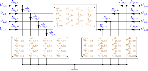
1. Data model
A line is an entry of the top-level line object, keyed by its string ID $\ell$. It carries exactly one impedance source: either a referenced linecode (per-metre matrices scaled by length) or inline absolute matrices.
| Field | Type | Unit | Req. | Description |
|---|---|---|---|---|
bus_from, bus_to | string | – | ✔ | Endpoint bus IDs $i$, $j$ |
terminal_map_from | string[] | – | ✔ | Conductor→terminal map at bus_from, $\textcolor{purple}{\mathbf{N}_{\ell i}}$ |
terminal_map_to | string[] | – | ✔ | Conductor→terminal map at bus_to, $\textcolor{purple}{\mathbf{N}_{\ell j}}$ |
linecode | string | – | (one-of) | Linecode ID (per-metre matrices) |
length | number | m | (with linecode) | Line length $\textcolor{red}{L_\ell}$ |
R_series_k_j, X_series_k_j | number | Ω | (one-of) | Inline absolute series impedance entries |
G_from_k_j, B_from_k_j | number | S | Inline from-side shunt admittance entries | |
G_to_k_j, B_to_k_j | number | S | Inline to-side shunt admittance entries | |
i_max | number[] | A | Per-conductor current-magnitude limit (overrides linecode) | |
s_max | number[] | VA | Per-conductor apparent-power limit (overrides linecode) |
The oneOf schema rule requires either linecode + length or at least R_series_1_1 + X_series_1_1 inline (and then no linecode).
Linecode
A linecode $c$ stores per-metre matrices shared across lines of the same type.
| Field | Type | Unit | Req. | Description |
|---|---|---|---|---|
R_series_k_j, X_series_k_j | number | Ω/m | ✔ | Per-metre series impedance $\mathfrak{R},\mathfrak{I}(\textcolor{brown}{\mathbf{Z}^{\text{s}}_c})$ |
G_from_k_j, G_to_k_j | number | S/m | Per-metre shunt conductance | |
B_from_k_j, B_to_k_j | number | S/m | Per-metre shunt susceptance | |
i_max | number[] | A | Per-conductor current limit $\textcolor{red}{\mathbf{I}^{\max}_c}$ | |
s_max | number[] | VA | Per-conductor apparent-power limit |
2. Input symbols
| Field | Symbol | Notes |
|---|---|---|
linecode R_series, X_series | $\textcolor{brown}{\mathbf{Z}^{\text{s}}_c}=\mathbf{R}+\textcolor{brown}{j}\mathbf{X}$ | Ω/m matrix |
linecode G/B_from, G/B_to | $\textcolor{brown}{\mathbf{Y}^{\text{sh}}_c}=\mathbf{G}+\textcolor{brown}{j}\mathbf{B}$ | S/m matrix |
length | $\textcolor{red}{L_\ell}$ | metres |
line R_series/X_series, G/B_* | $\textcolor{brown}{\mathbf{Z}^{\text{s}}_\ell},\ \textcolor{brown}{\mathbf{Y}^{\text{sh}}_{\ell ij}},\ \textcolor{brown}{\mathbf{Y}^{\text{sh}}_{\ell ji}}$ | Ω, S (absolute) |
i_max | $\textcolor{red}{\mathbf{I}^{\max}_{\ell ij}}$ | per conductor |
s_max | $\textcolor{red}{\mathbf{S}^{\max}_{\ell ij}}$ | per conductor |
Parameter construction
The line's series impedance and shunt admittances come from one source:
\[\text{linecode: }\quad \textcolor{brown}{\mathbf{Z}^{\text{s}}_\ell} = \textcolor{brown}{\mathbf{Z}^{\text{s}}_c}\,\textcolor{red}{L_\ell}, \qquad \textcolor{brown}{\mathbf{Y}^{\text{sh}}_{\ell ij}} = \textcolor{brown}{\mathbf{Y}^{\text{sh}}_{\ell ji}} = \tfrac{1}{2}\,\textcolor{brown}{\mathbf{Y}^{\text{sh}}_c}\,\textcolor{red}{L_\ell};\]
or the inline absolute matrices are used directly (never scaled by length). Inline data permits independent from- and to-side shunts $\textcolor{brown}{\mathbf{Y}^{\text{sh}}_{\ell ij}}\neq\textcolor{brown}{\mathbf{Y}^{\text{sh}}_{\ell ji}}$.
3. Variables
A line has $n_\ell = |\textcolor{purple}{\mathbf{N}_{\ell i}}|$ conductors. The series current flowing from $i$ toward $j$ is the independent unknown:
\[\textcolor{blue}{\mathbf{I}^{\text{s}}_{\ell ij}} \in \mathbb{C}^{n_\ell}.\]
The terminal current $\textcolor{blue}{\mathbf{I}_{\ell ij}}$ (what enters the bus's KCL) and the shunt current $\textcolor{blue}{\mathbf{I}^{\text{sh}}_{\ell ij}}$ are the other line currents; the equalities of part 4 relate them to $\textcolor{blue}{\mathbf{I}^{\text{s}}_{\ell ij}}$ and the bus voltages.
4. Equality constraints
Ohm's law (series voltage drop)
Across the series impedance, for the forward orientation $\ell ij$:
\[\textcolor{blue}{\mathbf{U}_j}[\textcolor{purple}{\mathbf{N}_{\ell j}}] = \textcolor{blue}{\mathbf{U}_i}[\textcolor{purple}{\mathbf{N}_{\ell i}}] - \textcolor{brown}{\mathbf{Z}^{\text{s}}_\ell}\,\textcolor{blue}{\mathbf{I}^{\text{s}}_{\ell ij}}.\]
The impedance matrix is full: off-diagonal entries couple the voltage drop on one conductor to the current in another.
Shunt currents
Each $\Pi$ half-section draws a current set by its admittance and the local bus voltage:
\[\textcolor{blue}{\mathbf{I}^{\text{sh}}_{\ell ij}} = \textcolor{brown}{\mathbf{Y}^{\text{sh}}_{\ell ij}}\,\textcolor{blue}{\mathbf{U}_i}, \qquad \textcolor{blue}{\mathbf{I}^{\text{sh}}_{\ell ji}} = \textcolor{brown}{\mathbf{Y}^{\text{sh}}_{\ell ji}}\,\textcolor{blue}{\mathbf{U}_j}.\]
Terminal current and series-current conservation
The current entering the line at each bus is the series current plus that end's shunt current, and the two directional series currents are equal and opposite:
\[\textcolor{blue}{\mathbf{I}_{\ell ij}} = \textcolor{blue}{\mathbf{I}^{\text{s}}_{\ell ij}} + \textcolor{blue}{\mathbf{I}^{\text{sh}}_{\ell ij}}, \qquad \textcolor{blue}{\mathbf{I}_{\ell ji}} = \textcolor{blue}{\mathbf{I}^{\text{s}}_{\ell ji}} + \textcolor{blue}{\mathbf{I}^{\text{sh}}_{\ell ji}}, \qquad \textcolor{blue}{\mathbf{I}^{\text{s}}_{\ell ij}} + \textcolor{blue}{\mathbf{I}^{\text{s}}_{\ell ji}} = \mathbf{0}.\]
The terminal currents $\textcolor{blue}{\mathbf{I}_{\ell ij}},\textcolor{blue}{\mathbf{I}_{\ell ji}}$ are the contributions this line makes to KCL at buses $i$ and $j$ (see Buses §4).
5. Inequality constraints
Cartesian variable bounds
A box may be placed on the series-current variable $\textcolor{blue}{\mathbf{I}^{\text{s}}_{\ell ij}}$ to bound the search. Because the engineering limit constrains the total (terminal) current, the box on the series part is the limit inflated by the worst-case shunt contribution $\rho_k$ on that row:
\[|\mathfrak{R}(\textcolor{blue}{I^{\text{s}}_{\ell ij,k}})| \le \textcolor{red}{I^{\max}_{\ell ij,k}} + \rho_k, \qquad |\mathfrak{I}(\textcolor{blue}{I^{\text{s}}_{\ell ij,k}})| \le \textcolor{red}{I^{\max}_{\ell ij,k}} + \rho_k,\]
with $\rho_k \le \sum_{j'} |\textcolor{brown}{Y^{\text{sh}}_{\ell ij,kj'}}|\,\textcolor{red}{U^{\max}_{i,j'}}$ from the endpoint voltage caps. This is a solver-conditioning aid; it is implied by the engineering bound below.
Engineering bounds
Thermal current limit on the terminal current, at both ends, for all conductors including neutral:
\[\textcolor{blue}{\mathbf{I}_{\ell ij}}\circ(\textcolor{blue}{\mathbf{I}_{\ell ij}})^{*} \le \textcolor{red}{\mathbf{I}^{\max}_{\ell ij}}\!\circ\textcolor{red}{\mathbf{I}^{\max}_{\ell ij}}, \qquad \textcolor{blue}{\mathbf{I}_{\ell ji}}\circ(\textcolor{blue}{\mathbf{I}_{\ell ji}})^{*} \le \textcolor{red}{\mathbf{I}^{\max}_{\ell ij}}\!\circ\textcolor{red}{\mathbf{I}^{\max}_{\ell ij}}.\]
Apparent-power limit (optional, from s_max), with the terminal power $\textcolor{blue}{\mathbf{S}_{\ell ij}} = \textcolor{blue}{\mathbf{U}_i}\circ(\textcolor{blue}{\mathbf{I}_{\ell ij}})^{*}$:
\[\textcolor{blue}{\mathbf{S}_{\ell ij}}\circ(\textcolor{blue}{\mathbf{S}_{\ell ij}})^{*} \le \textcolor{red}{\mathbf{S}^{\max}_{\ell ij}}\!\circ\textcolor{red}{\mathbf{S}^{\max}_{\ell ij}}.\]
Per-line angle difference (optional va_diff_min/va_diff_max). For each conductor, with $\textcolor{blue}{z}=\textcolor{blue}{U_{i,\cdot}}\,(\textcolor{blue}{U_{j,\cdot}})^{*}=c+\textcolor{brown}{j}s$:
\[\tan(\textcolor{red}{\theta^{\Delta,\min}_\ell})\, c \ \le\ s \ \le\ \tan(\textcolor{red}{\theta^{\Delta,\max}_\ell})\, c.\]
6. Implementation in BMOPFTools
Realisation
- Rectangular Ohm's law. The complex KVL is stamped as its two real parts per conductor $k$ (
branch.jl:_add_line_constraints!): $\mathfrak{R}(\textcolor{blue}{U_i})-\mathfrak{R}(\textcolor{blue}{U_j}) = \sum_{j'}(\mathbf{R}_{kj'}\mathfrak{R}(\textcolor{blue}{I^{\text{s}}})-\mathbf{X}_{kj'}\mathfrak{I}(\textcolor{blue}{I^{\text{s}}}))$ and $\mathfrak{I}(\textcolor{blue}{U_i})-\mathfrak{I}(\textcolor{blue}{U_j}) = \sum_{j'}(\mathbf{R}_{kj'}\mathfrak{I}(\textcolor{blue}{I^{\text{s}}})+\mathbf{X}_{kj'}\mathfrak{R}(\textcolor{blue}{I^{\text{s}}}))$. - Shunt currents are not variables. Where part 4 writes $\textcolor{blue}{\mathbf{I}^{\text{sh}}}=\textcolor{brown}{\mathbf{Y}^{\text{sh}}}\textcolor{blue}{\mathbf{U}}$ as a current, the code introduces no variable for it. It builds the affine JuMP expression $\textcolor{brown}{\mathbf{Y}^{\text{sh}}}\textcolor{blue}{\mathbf{U}}$ (
shunt.jl:_shunt_current!) and substitutes it in place wherever $\textcolor{blue}{\mathbf{I}^{\text{sh}}}$ appears — the KCL contribution and the terminal-current limit. The terminal current $\textcolor{blue}{\mathbf{I}_{\ell ij}}=\textcolor{blue}{\mathbf{I}^{\text{s}}_{\ell ij}}+\textcolor{brown}{\mathbf{Y}^{\text{sh}}_{\ell ij}}\textcolor{blue}{\mathbf{U}_i}$ is thus an expression, not a variable. This is exact — it eliminates the shunt-current variables and their defining equalities analytically. - Series-current alias. Only the from-side series current is a variable (
cr_fr/ci_fr,variables.jl:_add_line_variables!); the conservation law $\textcolor{blue}{\mathbf{I}^{\text{s}}_{\ell ji}}=-\textcolor{blue}{\mathbf{I}^{\text{s}}_{\ell ij}}$ is applied by making the to-side anAffExpralias-cr_fr, so it is never a separate variable or equality. - Conductor counts of the impedance matrix and both terminal maps must match exactly; a mismatch is refused (
E.INT.LINE_DIM_MISMATCH), never truncated. - Cartesian box is
_limit_current_box!inbranch.jl, added only when every voltage cap feeding the row is known. The thermal/apparent-power limits are the quadratics on the total-current and total-power expressions; the angle limit isbranch.jl:_add_line_angle_constraints!.
Source map
| Constraint | Code location |
|---|---|
| Series current variable | variables.jl:_add_line_variables! |
| Impedance / shunt construction | data_utils.jl:_line_z_matrix, _line_pi_shunt |
| Ohm's law (rectangular) | branch.jl:_add_line_constraints! |
| Shunt-current expression (substituted) | shunt.jl:_shunt_current! |
| KCL contributions | branch.jl:_add_line_constraints! (_kcl_add!) |
| Thermal / apparent-power limits | branch.jl:_add_line_constraints! |
| Series-current box | branch.jl (_limit_current_box!) |
| Per-line angle limit | branch.jl:_add_line_angle_constraints! |
Reconciliation notes (data model)
The PDF's line object lists only length, linecode, bus_from/to, terminal_map_from/to. The schema and code also support inline absolute impedance matrices (R_series_k_j, …, an alternative to linecode) and per-line i_max/s_max overrides of the linecode's ratings. Both ratings follow the precedence line override → linecode → unconstrained (applied independently to i_max and s_max), and both are enforced natively by the OPF — the current cone I∘I* ≤ I_max∘I_max and the ground-referenced per-conductor apparent-power cone S∘S* ≤ S_max∘S_max with S = U∘conj(I). The binding one can change with voltage, so the pair is not mathematically redundant, but declaring both is usually an engineering duplication; current is the source of truth for conductors and the neutral entry of s_max is degenerate (U_n ≈ 0). See current vs. apparent-power limits.
The PDF assumes symmetric half-shunts $\textcolor{brown}{\mathbf{Y}^{\text{sh}}_{\ell ij}}=\textcolor{brown}{\mathbf{Y}^{\text{sh}}_{\ell ji}}$. The code supports independent G_from/B_from vs G_to/B_to, so the two ends may differ; the symmetric case is the special case of equal fields.